About This Book

Most LLM applications shipping to production today run 10–50x more expensively than they need to. Latency is higher than users will tolerate, infrastructure costs are higher than the business can sustain, and the gap between a promising demo and a reliable product remains stubbornly wide.

The problem is not the model. The problem is everything around the model: context that is too large, prompts that are reprocessed on every call, tasks routed to expensive models that cheaper ones handle just as well, agent loops with no bounds.

This book is the engineering layer above model selection. It defines six governing laws of production LLM systems and applies them across fourteen chapters covering inference mechanics, context architecture, execution strategy, and deployment operations. Every technique is grounded in production results — what actually breaks at scale, not what looks good in benchmarks.

Target reader: Senior engineers, platform engineers, and technical leads responsible for the latency, cost, and reliability of LLM-powered systems. You already know what LLMs are. This book shows you how to ship them.

---

Contents

---

The Six Laws of Production LLM Systems

Every chapter in this book applies one or more of these laws. They are the governing constraints of every LLM system in production.

Context Engineering Defined

Context engineering is the discipline of designing and optimizing everything sent to a language model — system prompts, retrieved data, conversation history, tool definitions — to minimize cost and latency while preserving response quality.

It is not prompt engineering. Context engineering is the engineering layer above: deciding what data to include, how to structure it, what to cache, what to filter, and when to route to a different model.

If prompt engineering is writing a good email, context engineering is designing the mail system.

What Happens When You Call the API

A typical API call:

response = client.messages.create(
    model="claude-sonnet-5",
    max_tokens=1024,
    system="You are a helpful math tutor for grade 5...",
    messages=[
        {"role": "user", "content": "How do I add fractions?"}
    ]
)

Between client.messages.create() and the response, four distinct stages execute — each with different performance characteristics and optimization opportunities.

Step 1: Tokenization

Text enters the model as tokens — chunks typically representing 3-4 characters in English. The sentence "How do I add fractions?" becomes roughly seven tokens.

Tokens are the fundamental unit of LLM economics — pricing, latency metrics, and every optimization in this book operate at the token level.

Token Counting Rules of Thumb

1 token ≈ 4 characters ≈ 0.75 words in English prose

A 2,000-word document ≈ 2,700 tokens

Code tokenizes at ~2-3 characters per token (less efficient than prose)

Structured data is less efficient: {"name": "Alice"} costs 10 tokens; name: Alice costs 4

Step 2: Prefill — Processing the Input

Once tokenized, the entire input — system prompt, conversation history, user message, tool definitions — enters the model in a single batch. The model processes all tokens simultaneously in the prefill phase.

During prefill, the model transforms each input token into internal Key and Value vectors. This is computationally intensive — heavy matrix multiplications — but because all input tokens are known upfront, the work is parallelized across the GPU's thousands of cores.

Reference latencies for a 70B parameter model on NVIDIA A100 (312 TFLOPS; newer accelerators are faster in absolute terms, but the scaling pattern is identical):

Input Size	Prefill Time	Relative to 1K	Notes
1,000 tokens	~0.45 seconds	1x	Linear regime
5,000 tokens	~2.25 seconds	5x	Linear regime
10,000 tokens	~4.5 seconds	10x	Linear regime
50,000 tokens	~27-30 seconds	60-67x	Attention overhead visible
100,000 tokens	~65-90 seconds	145-200x	Quadratic attention dominates

At short-to-moderate contexts (<16K), feedforward computation dominates and scaling is effectively linear (~0.45ms per token). At longer contexts, the O(n²) attention computation becomes the bottleneck. FlashAttention and related optimizations reduce memory overhead but do not eliminate the compute scaling. Managed API latencies differ in absolute terms but follow the same scaling pattern.

The difference between a 5,000-token context and a 50,000-token context is roughly twenty-five seconds of waiting before the model generates a single output token. That is not network latency or slow code. It is compute: more input means more computation. This is Law 1 (The Prefill Law) in action.

Step 3: Decode — Generating the Response

Once prefill completes, the model produces output tokens one at a time. This is the decode phase. Decode is inherently sequential — the model must produce token 1 before token 2, because each token's probability depends on every token before it.

Decode has a fundamentally different performance profile. Prefill is compute-bound (GPU busy calculating). Decode is memory-bound (GPU spends most time loading model weights from memory). Each output token takes roughly the same time to generate, regardless of input length.

Model Class	Approximate Decode Speed	1,000 Tokens Takes
70B (e.g., Llama 70B on A100)	~11 tokens/second	~90 seconds
Medium (~30B, API mid-tier)	~30-40 tokens/second	~25-33 seconds
Small (~8B, API fast tier)	~60-80 tokens/second	~12-17 seconds

Decode speed is approximately constant with respect to input length. At very long contexts (100K+), KV cache reads add minor overhead.

Step 4: Streaming

Streaming exposes the two-phase architecture directly to the user:

• The pause before the first word — the prefill phase. Longer context means longer pause.
• The speed at which words appear — the decode phase. Roughly constant regardless of context length.

These map to two critical metrics:

Metric	What It Measures	Controlled By
Time to First Token (TTFT)	Delay before response starts	Prefill time (input length)
Tokens per Second (TPS)	Speed of streaming output	Decode rate (model + hardware)

TTFT is the metric users feel most acutely. 200ms feels instant. 2 seconds feels slow. 20 seconds feels broken. Since TTFT is driven by prefill, which scales with input length, context engineering directly controls user-perceived responsiveness. This is Law 1 applied to user experience.

The Two Phases: A Concrete Comparison

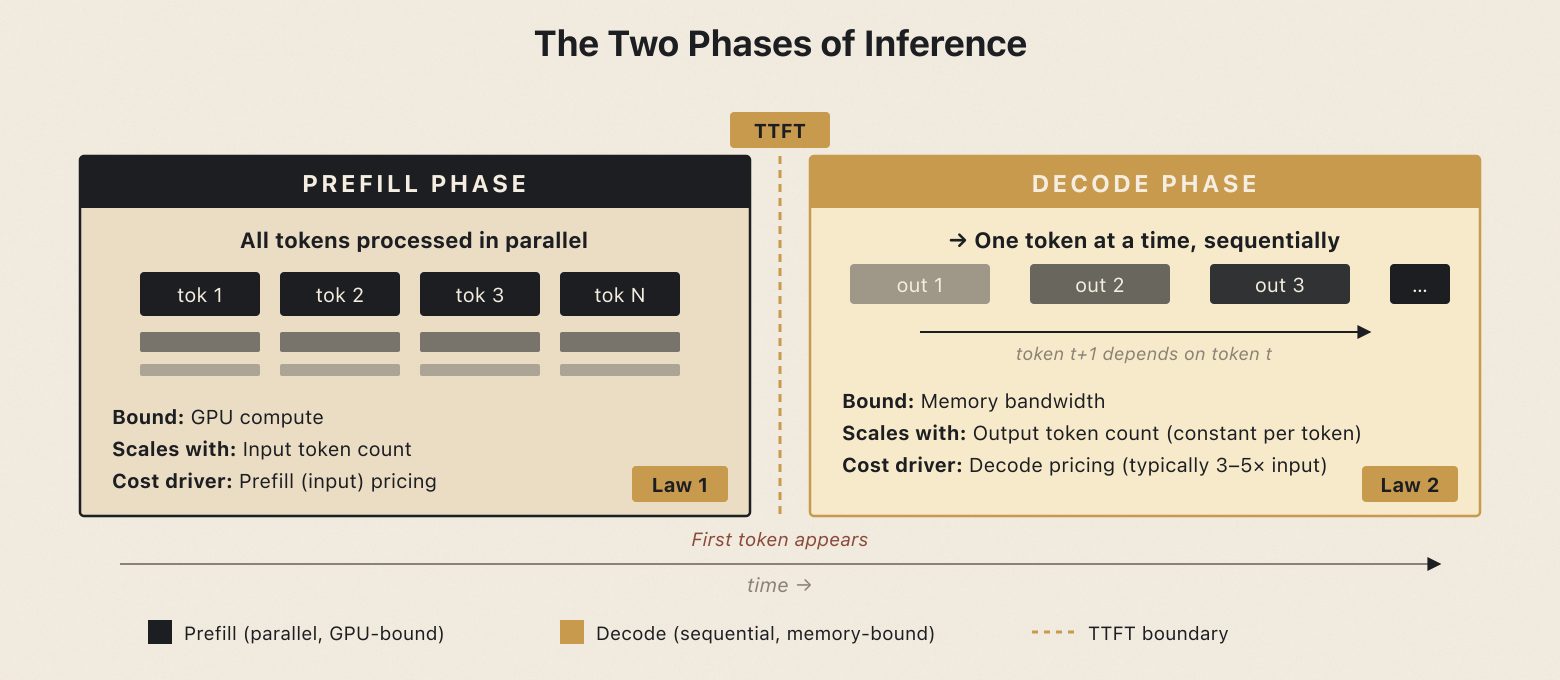
Baseline: mid-tier model (Sonnet-class), managed API, 500-token response.

	Bloated Agent	Optimized Agent
Input tokens	50,000	5,000
Output tokens	500	500
TTFT (prefill)	~8 seconds	~0.8 seconds
Decode time	~14 seconds	~14 seconds
Total time	~22 seconds	~14.8 seconds
Improvement	—	33% faster, 10x less input cost

Input reduced by 90%. Total response time dropped by a third. Decode time unchanged. Response identical in length and quality. The user receives it 7 seconds sooner, with sub-second TTFT instead of eight seconds of blank screen.

At typical API pricing, 45,000 eliminated input tokens save money on every request — across thousands of daily users, the difference between a sustainable product and one that bleeds money.

What Is in the Context Window

Typical context breakdown by application archetype:

Component	Simple Chatbot	RAG Application	Tool-Using Agent
System prompt	800 tokens	2,000 tokens	3,500 tokens
Tool definitions	—	—	8,000 tokens
Retrieved context	—	12,000 tokens	6,000 tokens
Conversation history	1,500 tokens	3,000 tokens	2,500 tokens
User message	100 tokens	200 tokens	150 tokens
Total input	2,400	17,200	20,150
User message as % of total	4.2%	1.2%	0.7%

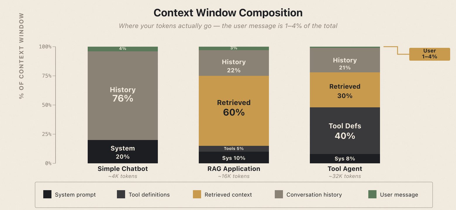
Two observations:

1. The user's actual question is typically 1-4% of total input (often under 1% for tool-heavy agents). The other 96-99% is context: instructions, data, history, tool definitions.
2. A large portion of that context is identical across every request. System prompt and tool definitions never change. This static content gets re-processed from scratch on every API call — unless you act on it.

The dynamic content — retrieved context, conversation history — is often larger than necessary for any given query. A user asking "What's my next assignment?" does not need 12,000 tokens of course material. Sending it all is the default behavior of most RAG implementations, and it is where the largest optimization opportunities exist.

The Optimization Stack: Preview

Five optimization layers, each targeting a different point in the pipeline:

Layer	Strategy	What It Does	Chapter
1	Data Engineering	Restructure data for fewer tokens	Ch 3
2	Query-Aware Filtering	Send only what is relevant to this query	Ch 4
3	Prompt Caching	Skip re-processing static portions	Ch 5
4	Prompt Simplification	Reduce instruction and output overhead	Ch 6
5	Architecture	Route queries, parallelize calls, right-size models	Ch 7-9

These layers compound. Applying all five to a production agent typically yields 85-95% reduction in token usage and drops latency from tens of seconds to single digits.

A Note on Real-World Latency

The latencies in this chapter represent raw computation. Actual API latency includes network round-trips, request queuing, and provider-side optimizations. Measured numbers differ from theoretical calculations, but proportional relationships hold — a 10x input reduction yields substantial real-world TTFT improvement.

What You Now Know

The core insight: your LLM application spends most of its time and money processing the input, not generating the answer. The prefill phase — processing system prompt, retrieved context, conversation history — is the bottleneck. The decode phase is largely fixed.

Every unnecessary token in your input costs three times over: API fees, user-facing latency, and infrastructure capacity. Context engineering eliminates that waste — not by sending less, but by sending smarter: the right data, in the right format, cached where possible, filtered for relevance, and routed to the right model.